Gaussian Process Emulator

This notebook contains basic working examples of fitting and running inference using Gaussian Processes (GPs) as the base estimator model in twinLab.

An in-depth introductory review of GPs can be found at Rasmussen and Williams (2006).

This notebook will cover:

• Basic syntax

• Detrending data

• Specifying a covarance module

# Third-party imports
import numpy as np
import pandas as pd
import matplotlib.pyplot as plt

# twinLab import
import twinlab as tl

Problem Formulation

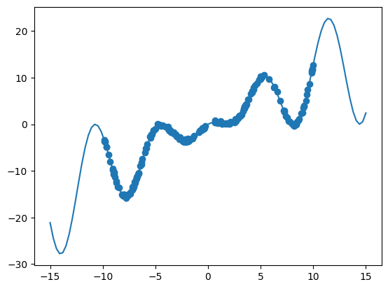
As a start, we will solve a simple regression problem with one input and one output.

# The true function
def oscillator(x):
    return np.cos((x - 5) / 2) ** 2 * x * 2


X = np.linspace(-15, 15, 100)[:, np.newaxis]
y = oscillator(X)  # Arrange outputs as feature columns

n_data = 200
X_data = np.random.uniform(-10, 10, size=n_data)
y_data = oscillator(X_data) + np.random.normal(scale=0.2, size=X_data.shape)

plt.plot(X, y)
plt.scatter(X_data, y_data)
plt.show()

Datasets must be data presented as a pandas.DataFrame object, or a filepaths which points to a csv file that can be parsed to a pandas.DataFrame object. Both must be formatted with clearly labelled columns. Here, we will label the input (predictor) variable x and the output variable y. In twinlab, data is expected to be in column-feature format, meaning each row represents a single data sample, and each column represents a data feature.

# Convert to dataframe
df = pd.DataFrame({"x": X_data, "y": y_data})
df.head()

	x	y
0	3.651887	4.344898
1	-9.052743	-9.454922
2	-9.649020	-4.871539
3	8.479235	0.503219
4	-5.774704	-4.326750

# Define the name of the dataset
dataset_id = "BasicGP_Data"

# Upload the dataset to the cloud
dataset = tl.Dataset(id=dataset_id)
dataset.upload(df)

Basic Emulator Workflow

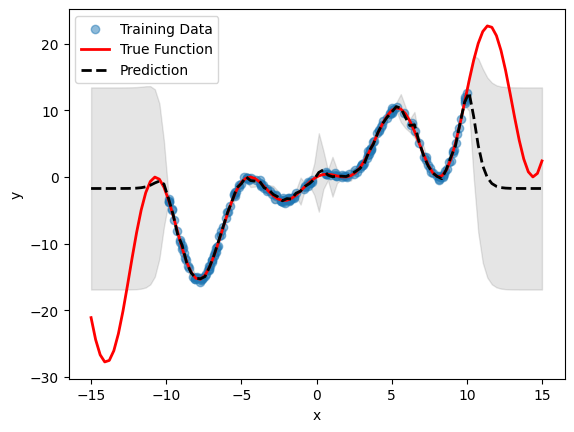
By default, a Emulator object will try to fit a Gaussian Process with a Constant Mean and a Matern 5/2 covariance kernel to the data. This is done with the basic syntax shown below.

Note: the train_test_ratio parameter determines how many data samples in df to use for fitting the model. E.g. if train_test_ratio=0.4, then 40% of the samples in df are used for fitting, and the remaining data is used for testing. The data reserved for testing is used to assess the performance of the model.

# Initialise emulator
emulator_id = "BasicGP"

emulator = tl.Emulator(id=emulator_id)

# Define the training parameters for your emulator
params = tl.TrainParams(
    train_test_ratio=0.75, estimator="gaussian_process_regression"
)

# Train the mulator using the train method
emulator.train(dataset=dataset, inputs=["x"], outputs=["y"], params=params)

# Plot inference results
df_pred = emulator.predict(pd.DataFrame(X, columns=["x"]))
result_df = pd.concat([df_pred[0], df_pred[1]], axis=1)
df_mean, df_stdev = result_df.iloc[:, 0], result_df.iloc[:, 1]
y_mean, y_stdev = df_mean.values, df_stdev.values

plt.fill_between(
    X.flatten(),
    (y_mean - 1.96 * y_stdev).flatten(),
    (y_mean + 1.96 * y_stdev).flatten(),
    color="k",
    alpha=0.1,
)

plt.scatter(df["x"], df["y"], alpha=0.5, label="Training Data")
plt.xlabel("x")
plt.ylabel("y")

plt.plot(X, y, c="r", linewidth=2, label="True Function")
plt.plot(X, y_mean, c="k", linewidth=2, linestyle="dashed", label="Prediction")
plt.legend()
plt.show()

Detrending Data

A standard data processing task before fitting a model to data is (linear) detrending: here, the linear non-stationary information about the data is subtracted from the data. This may help with subsequent model fitting.

In Emulator, this is achieved simply with the keyword detrend provided to the estimator_params argument, inside the TrainParams, during initialisation. This results in the following code:

# Initialise emulator
emulator_id = "DetrendingGP"

detrending_emulator = tl.Emulator(id=emulator_id)

# Define the estimator params and allow detrending of data
estimator_params = tl.EstimatorParams(detrend=True)

# Define the training parameters for your emulator
params = tl.TrainParams(
    train_test_ratio=0.75,
    estimator="gaussian_process_regression",
    estimator_params=estimator_params,
)

# Train the emulator using the defined parameters
detrending_emulator.train(
    dataset=dataset, inputs=["x"], outputs=["y"], params=params, verbose=True
)

Model DetrendingGP has begun training.
Training complete!

# Plot inference results
df_pred = emulator.predict(pd.DataFrame(X, columns=["x"]))
result_df = pd.concat([df_pred[0], df_pred[1]], axis=1)
df_mean, df_stdev = result_df.iloc[:, 0], result_df.iloc[:, 1]
y_mean, y_stdev = df_mean.values, df_stdev.values

plt.fill_between(
    X.flatten(),
    (y_mean - 1.96 * y_stdev).flatten(),
    (y_mean + 1.96 * y_stdev).flatten(),
    color="k",
    alpha=0.1,
)

plt.scatter(df["x"], df["y"], alpha=0.5, label="Training Data")
plt.xlabel("x")
plt.ylabel("y")

plt.plot(X, y, c="r", linewidth=2, label="True Function")
plt.plot(X, y_mean, c="k", linewidth=2, linestyle="dashed", label="Prediction")
plt.legend()
plt.show()

Note the difference in the mean prediction of the detrended model compared to the standard model without detrending (from the previous section). The prediction is automatically re-trended during inference, so no need for any other operations.

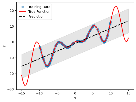
Specifying a Covariance Kernel

In some cases, it may be desirable to specify a covariance module for the GP. The user may have some belief that the process is linear in nature, or may contain a combination of periodic signals at different length-scales, or may want to specifically account for short-time noise in the data.

Emulator allows the user to do this, via the covar_module keyword provided to the estimator_params dictionary. Currently, the kernels are provided as 3-character uppercase strings. The list of possible kernels are:

• "LIN": Linear kernel

• "M12": Matern 1/2 kernel

• "M32": Matern 3/2 kernel

• "M52": Matern 5/2 kernel

• "PER": Periodic kernel

• "RBF": Radial Basis Function kernel

• "RQF": Rational Quadratic Kernel

Additionally, the kernels can be composed using brackets and + or * string operators. For example:

• "LIN+PER"

• "(M52*PER)+RQF

# Initialise emulator
emulator_id = "LinearGP"

linear_emulator = tl.Emulator(id=emulator_id)

# Define the estimator params with a covariance function
estimator_params = tl.EstimatorParams(covar_module="LIN")

# Define the training parameters for your emulator
params = tl.TrainParams(
    train_test_ratio=0.75,
    estimator="gaussian_process_regression",
    estimator_params=estimator_params,
)

# Train the emulator using the defined parameters
linear_emulator.train(dataset=dataset, inputs=["x"], outputs=["y"], params=params)

# Plot inference results
df_pred = linear_emulator.predict(pd.DataFrame(X, columns=["x"]))
result_df = pd.concat([df_pred[0], df_pred[1]], axis=1)
df_mean, df_stdev = result_df.iloc[:, 0], result_df.iloc[:, 1]
y_mean, y_stdev = df_mean.values, df_stdev.values

plt.fill_between(
    X.flatten(),
    (y_mean - 1.96 * y_stdev).flatten(),
    (y_mean + 1.96 * y_stdev).flatten(),
    color="k",
    alpha=0.1,
)

plt.scatter(df["x"], df["y"], alpha=0.5, label="Training Data")
plt.xlabel("x")
plt.ylabel("y")

plt.plot(X, y, c="r", linewidth=2, label="True Function")
plt.plot(X, y_mean, c="k", linewidth=2, linestyle="dashed", label="Prediction")
plt.legend()
plt.show()

# Delete campaigns and dataset
tl.delete_campaign("BasicGP")
tl.delete_campaign("DetrendingGP")
tl.delete_campaign("LinearGP")

tl.delete_dataset(dataset_id)